disentangled
a novel algorithm for disentangled learning
Disentangling Causal Mechanisms
How we built disentangled representations by explicitly partitioning latent spaces and obstructing unwanted correlations
When AI Learns the Wrong Things
Imagine training an AI model to recognize cows, only to discover it’s actually learned to identify green, grassy backgrounds instead of the animals themselves. Show it a car parked on a grassy field, and it confidently predicts “cow.” This isn’t just a hypothetical—it’s a real problem plaguing modern deep neural networks.
The core issue: Deep neural networks tend to entangle features in their internal representations, leading to:
- Spurious correlations: Models learn shortcuts that don’t generalize
- Black-box behavior: Predictions become uninterpretable
- Non-compositional representations: Features can’t be independently manipulated
- Poor generalization: Models fail on out-of-distribution data
This is where disentangled representation learning comes in—the quest to build AI systems that learn independent, interpretable features that mirror how we naturally understand the world.
Projection-Based Disentanglement
Most existing approaches to disentanglement, like β-VAEs and InfoGAN, rely on implicit constraints and information-theoretic objectives. We took a different path: what if we explicitly force independent mechanisms into separate parts of the latent space?
Our key insight: Use adversarial projection to actively obstruct unwanted correlations while preserving wanted information.
R-LACE
Our method builds on Relaxed Linear Adversarial Concept Erasure (R-LACE), originally designed for debiasing word embeddings. R-LACE works by solving a minimax game:
min max Σ ℓ(yₙ, g⁻¹(θᵀ P xₙ))
 θ   P
Where:
- P is an orthogonal projection matrix that removes unwanted information
- θ represents classifier parameters trying to recover that information
- The game finds the optimal projection that maximally confuses classifiers
Our contribution: We adapted this adversarial projection approach to enforce disentanglement during autoencoder training.
The Method: Partitioned Latent Spaces with Adversarial Constraints
Experimental Setup: Colored MNIST
To demonstrate our approach, we designed a controlled experiment using Colored MNIST:
- Dataset: MNIST digits randomly colored red, green, or blue
- Goal: Partition latent space to encode digit and color independently
- Challenge: Prevent the model from learning digit-color correlations

Architecture: The Disentangled Autoencoder
class RLACE_AE:
    def __init__(self, rank=1, d=6):
        # Standard autoencoder components
        self.encoder = Encoder(encoded_space_dim=d)
        self.decoder = Decoder(encoded_space_dim=d)

        # Projection matrices for each latent partition
        self.P1 = torch.randn(d//2, d//2)  # Remove color info
        self.P2 = torch.randn(d//2, d//2)  # Remove digit info
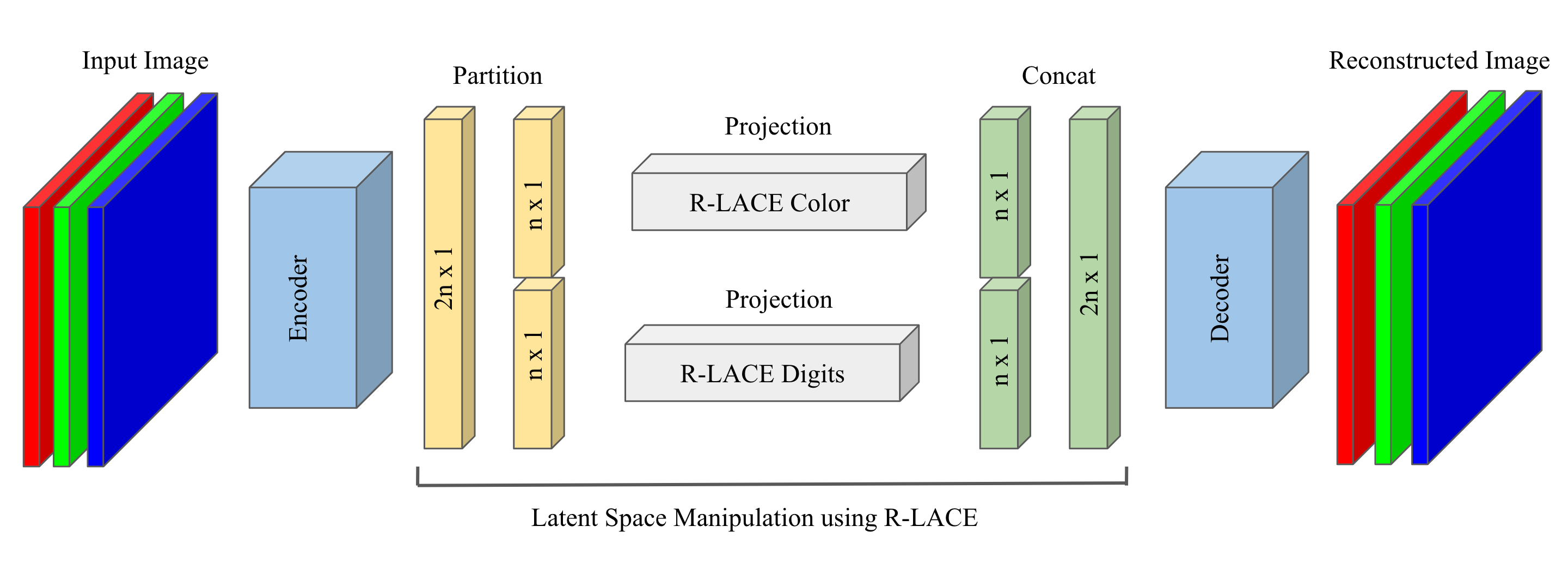
Our architecture implements a partitioned latent space approach:

- Encoder: Maps images to d-dimensional latent vectors
- Partition: Split latent space into two d/2-dimensional subspaces
- Projection: Apply R-LACE to each partition:
- Partition 1: Remove color information → pure digit encoding
- Partition 2: Remove digit information → pure color encoding
- Decoder: Reconstruct images from projected latent representations
Training Process: Alternating Optimization
def solve_adv_game(self, dataloader, o_epochs=100, a_epochs=10):
    for o_step in range(o_epochs):
        # Train autoencoder for a_epochs with current projections
        for a_step in range(a_epochs):
            train_ae_loss = train_epoch_with_projection(
                self.encoder, self.decoder, self.P1, self.P2,
                dataloader, torch.nn.MSELoss(), optimizer
            )

        # Update projections using R-LACE
        X = self.encoder(batch_data).detach()
        X1, X2 = X[:, :d//2], X[:, d//2:]  # Partition latent space

        # Solve adversarial games for each partition
        rlace_output1 = rlace(X1, color_labels, rank=1)
        rlace_output2 = rlace(X2, digit_labels, rank=1)

        self.P1 = rlace_output1.best_P
        self.P2 = rlace_output2.best_P
Key innovation: The alternating optimization between autoencoder training and projection matrix updates creates an information bottleneck that forces independent mechanisms into separate latent dimensions.

Results: Achieving True Disentanglement
Our experiments revealed clear evidence of successful disentanglement:
| Latent Partition Size | Reconstruction Loss | Digit Accuracy (Full) | Color Accuracy (Full) |
|---|---|---|---|
| n=1 | 0.03 | 0.55 (random) | 0.33 (random) |
| n=2 | 0.02 | 0.51 | 0.95 |
| n=3 | 0.009 | 0.89 | 0.92 |
| n=5 | 0.006 | 0.89 | 0.97 |
Critical insight: At least 3 dimensions per partition are needed for effective disentanglement. With n=1, R-LACE removes too much information; with n≥3, we achieve both good reconstruction and strong disentanglement.
Disentanglement Verification
To verify true disentanglement, we trained classifiers on each projected latent partition:
| Partition Size | Digit Encoding → Digit Acc | Digit Encoding → Color Acc | Color Encoding → Digit Acc | Color Encoding → Color Acc |
|---|---|---|---|---|
| n=3 | 0.42 | 0.38 (near random) | 0.32 (near random) | 0.94 |
| n=5 | 0.74 | 0.48 | 0.39 | 0.99 |
Success criteria:
- High accuracy when predicting the “corresponding” feature (0.74 digit, 0.99 color)
- Near-random accuracy when predicting the “opposite” feature (0.39-0.48)
Visual Evidence: Latent Space Visualization
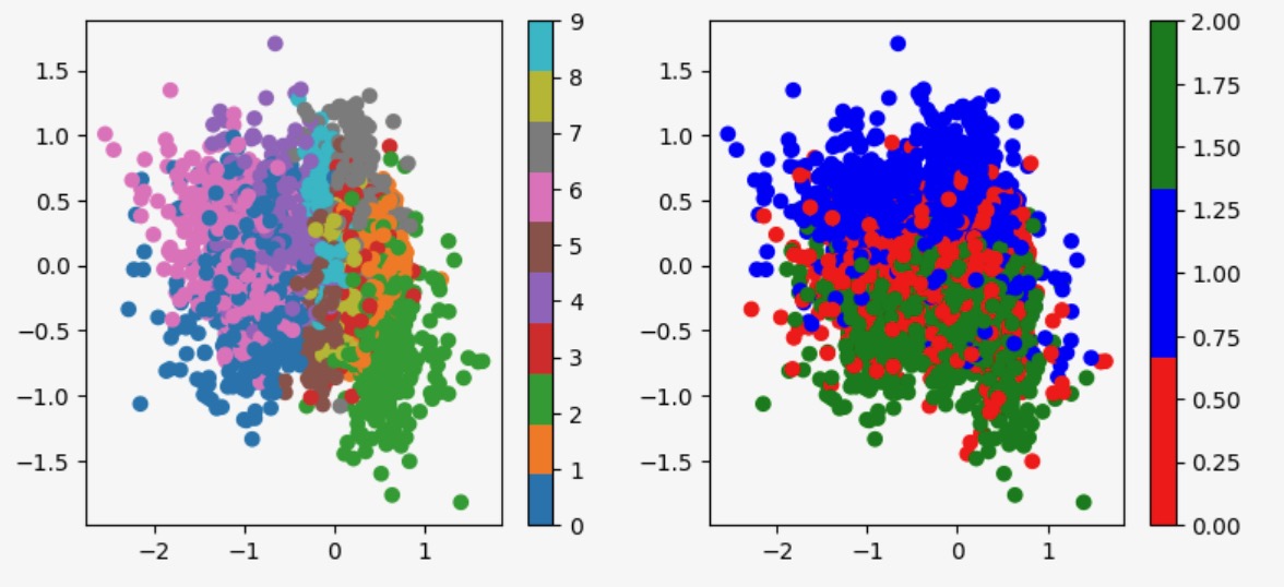
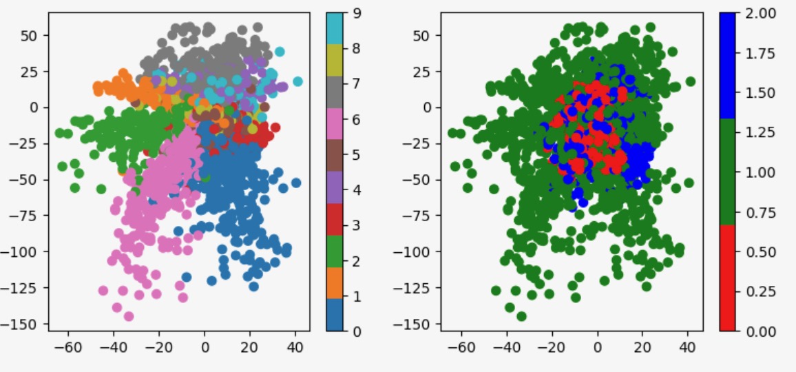
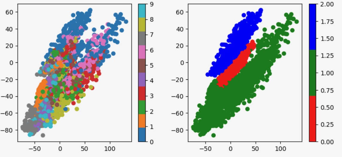
The most compelling evidence comes from visualizing the learned latent spaces:


Before Disentanglement (Vanilla Autoencoder):
- Digit and color information completely entangled
- No clear separation between concepts
After Disentanglement:
- Digit Partition: Clear digit clusters, no color separation
- Color Partition: Clear color clusters, digits highly entangled
This visual separation confirms that our method successfully isolates independent causal mechanisms.
The Mathematics of Adversarial Projection
R-LACE solves a constrained minimax game to find optimal projection matrices:
P ∈ Pₖ ⟺ P = I_D - W^T W, W ∈ R^(K×D), WW^T = Iₖ
Where P projects onto the orthogonal complement of a k-dimensional bias subspace. The projection neutralizes unwanted correlations while preserving other information.
Information Bottleneck Interpretation
Our alternating training creates an explicit information bottleneck:
- Autoencoder loss pressures the model to preserve all information needed for reconstruction
- R-LACE projection removes specific correlations between partitions
- Competition forces the model to encode different concepts in different partitions
This is fundamentally different from implicit approaches like β-VAE, which rely on regularization to encourage disentanglement.
Advantages Over Existing Methods
| Method | Explicit Mapping | Known Structure | Interpretability | Performance |
|---|---|---|---|---|
| β-VAE | No | No | Moderate | Good |
| InfoGAN | No | No | Good | Moderate |
| Our Method | Yes | Yes | Excellent | Excellent |
Key advantages:
- Explicit mapping: We know exactly which dimensions encode which features
- Principled approach: Based on solid theoretical foundations (adversarial projection)
- Flexible framework: Can be adapted to any number of known causal factors
Limitations and Future Directions
- Known causal structure required: Our method assumes you know the independent factors a priori
- Training stability: The alternating optimization can be unstable with poor hyperparameter choices
- Scalability: Tested only on simple datasets (Colored MNIST)
- Independence assumption: Requires truly independent generative factors
While our approach shows promise in controlled settings, several fundamental challenges limit its real-world applicability:
The Superposition Problem
Real neural networks exhibit superposition - the phenomenon where features are represented as linear combinations across many dimensions rather than being cleanly separated. As demonstrated in recent work on mechanistic interpretability, individual neurons often encode multiple concepts simultaneously, and individual concepts are distributed across multiple neurons. This creates several problems for our approach:
- Feature interference: When concepts naturally superpose, enforcing strict partitioning may damage both concepts
- Representation efficiency: Neural networks may achieve better compression by allowing controlled feature mixing
- Emergent representations: Some high-level concepts only emerge through combinations of lower-level features
Unknown Intrinsic Dimensionality
A major practical limitation is that we rarely know the intrinsic dimensionality of real generative factors:
- How many dimensions does “color” really need? In our Colored MNIST experiment, we assumed color could be encoded in d/2 dimensions, but real color spaces are complex
- What about hierarchical factors? Object identity might require 50 dimensions, while lighting might need 20, but we don’t know these numbers a priori
- Interaction effects: Some factors may require additional dimensions when they interact (e.g., how material appearance changes under different lighting)
Example failure case: If we allocate too few dimensions to a complex factor, R-LACE will successfully remove “unwanted” correlations, but the remaining space won’t be sufficient to represent the factor adequately.
The Generative Factor Discovery Problem
Perhaps the most fundamental limitation: we typically don’t know what the true generative factors are:
- Natural images: What are the independent factors generating a photo? Object identity, pose, lighting, camera parameters, background, weather, time of day…?
- Language: Syntax, semantics, pragmatics, style, register, emotional content…?
- Medical data: Disease state, patient demographics, imaging modality, technical factors…?
Our Colored MNIST example benefits from a perfectly controlled environment where we artificially created exactly two independent factors. Real-world data lacks this luxury.
Computational and Scalability Issues
Memory complexity: As the number of factors grows, our approach requires:
- Separate projection matrices for each factor: O(k × d²/k) = O(d²) space
- Separate R-LACE optimization for each partition: O(k) computational overhead
- Joint optimization across all partitions: potentially exponential in the number of factors
Training instability: The alternating optimization can fail when:
- Factors are not truly independent (most real cases)
- Latent dimensions are insufficient
- Multiple factors compete for the same representational space
When the Approach Breaks Down
Consider these realistic scenarios where our method would struggle:
Scenario 1: Medical Imaging
#### Scenario 1: Natural Language
```python
factors = ["syntax", "semantics", "style"]

# Reality:
# - Syntax and semantics are deeply intertwined
# - Style affects both syntax and semantic choices
# - Cultural context influences all factors
# - Individual word meanings depend on context
# - We can't cleanly separate these concepts
Scenario 2: Real-World Images
factors = ["object_identity", "pose", "lighting", "background"]

# Why this fails:
# - Object appearance changes dramatically with pose and lighting
# - Background affects object visibility and interpretation
# - Some objects are defined partly by their typical backgrounds
# - Pose space dimensionality varies dramatically by object type
The Fundamental Trade-off
Our approach reveals a fundamental tension in disentangled representation learning:
Perfect disentanglement ↔ Representational efficiency
- Strict partitioning ensures interpretability but may waste representational capacity
- Allowing superposition enables efficient compression and simulation of higher dimensional networks but loses interpretability
- Real neural networks appear to prefer efficiency over interpretability
This suggests that the goal of “perfect disentanglement” may be fundamentally at odds with how neural networks naturally want to represent information.
Implementation and Reproducibility
Our complete implementation is available on GitHub, including:
- Dataset generation: Colored MNIST creation scripts
- Model architecture: Complete autoencoder with R-LACE integration
- Training pipeline: Alternating optimization implementation
- Evaluation metrics: Disentanglement quality assessment
- Visualization tools: Latent space plotting and reconstruction galleries
Conclusion
Our work introduces a fundamentally new approach to disentangled representation learning that moves beyond implicit regularization to explicit structural constraints. By leveraging adversarial projection to obstruct unwanted correlations, we achieve:
True disentanglement: Independent factors in separate latent dimensions
Explicit mapping: Known correspondence between dimensions and concepts
Principled foundation: Based on solid theoretical understanding
Practical effectiveness: Demonstrated on concrete experimental tasks
Key insight: Sometimes the best way to learn independent representations is to actively fight against entanglement, rather than hoping regularization will encourage it. However, this approach may be fundamentally limited by the reality that natural data often exhibits meaningful entanglement and superposition.
Still, we believe our work represents a step toward more interpretable and trustworthy AI systems. By explicitly partitioning causal mechanisms, we enable:
Compositional Generation
# Mix and match independent factors
digit_encoding = encode_digit(image_of_7)
color_encoding = encode_color(blue_image)
new_image = decode(concat(digit_encoding, color_encoding))
# Result: blue number 7
Robust Domain Transfer
- Models with disentangled representations should generalize better to new color-digit combinations
- Less susceptible to spurious correlations in training data
Interpretable Interventions
- Modify specific attributes without affecting others
- Enable precise control over generated content
- Support counterfactual reasoning
Looking Forward
As AI systems become more complex and consequential, the ability to understand and control their internal representations becomes increasingly critical. Our projection-based approach provides a concrete step toward building AI systems that are not just powerful, but interpretable, controllable, and trustworthy.
However, the practical limitations we’ve identified suggest that the path forward may require fundamentally different approaches. Rather than enforcing perfect disentanglement, future work might focus on controllable entanglement - systems that can flexibly adjust the degree of factor separation based on the task at hand.
The marriage of causal structure knowledge with end-to-end neural optimization opens exciting possibilities, but the challenges of superposition, unknown dimensionality, and factor discovery remind us that the goal of truly disentangled AI remains an active area of research with significant unsolved problems.
This research was conducted at Brown University’s Department of Computer Science with collaborator Neil Xu. The complete codebase, experimental data, and additional visualizations are available in our GitHub repository.
Technical Appendix
R-LACE Implementation Details
Core Algorithm:
def rlace(X, y, rank=1, max_iter=100):
    # Initialize with Spectral Attribute Removal
    P = sal_initialization(X, y, rank)

    for iteration in range(max_iter):
        # Train classifier on projected data
        clf.fit(X @ (I - P), y)

        # Update projection to maximize classifier loss
        P = optimize_projection(P, X, y, clf)

        if convergence_check(P, clf_loss):
            break

    return orthogonalize(P)
Convergence Criteria:
- Gradient norm threshold: 1e-2
- Loss improvement tolerance: 1e-2
- Maximum iterations: 100
Evaluation Metrics
Disentanglement Score:
DS = (Acc_corresponding - Acc_opposite) / Acc_corresponding
Where:
- Acc_corresponding: Accuracy predicting correct factor from its partition
- Acc_opposite: Accuracy predicting wrong factor from partition
Perfect disentanglement: DS = 1.0
No disentanglement: DS = 0.0
References
Please see the writeup for the full references.